HEALTHCARE ORGANISATION CLINICAL ANALYTICS REPORT

Health Data Analytics

Stroke Prediction
& Risk Modelling

An end-to-end clinical analytics investigation into patient characteristics, risk factors, and predictive modelling of stroke likelihood across 5,110 patient records.

PREPARED BY Freda Erinmwingbovo

ROLE Health Data Analyst

DATE March 2026

RECORDS ANALYSED 5,110 Patient Records

1 About This Report

This report documents the end-to-end development and deployment of a stroke prediction model on behalf of a leading healthcare organisation. Working in the role of a health data analyst, the analysis covers the full analytical pipeline, from raw data ingestion and preprocessing through to exploratory analysis, model building, evaluation, and clinical deployment.

According to the World Health Organization (WHO), stroke is the second leading cause of death globally, accounting for approximately 11% of all deaths worldwide. Early identification of at-risk patients offers a critical window for intervention. This project leverages a dataset of 5,110 patient records across 11 clinical and demographic features to build a validated predictive model that can support frontline clinical decision-making.

2 Introduction and Data Loading

2.1 Background & Objectives

A leading healthcare organisation has identified a concerning trend, an increasing number of patients are being diagnosed with strokes across its facilities. In response, the organisation has commissioned this analytical project to build a validated predictive model capable of identifying patients at elevated risk of stroke, enabling earlier clinical intervention and more targeted preventive care.

According to the World Health Organization (WHO), stroke is the second leading cause of death globally, responsible for approximately 11% of all deaths. The consequences of a stroke extend beyond mortality. Survivors frequently face long-term disability, cognitive impairment, and reduced quality of life. Early identification of at-risk patients offers a critical window for intervention that can meaningfully alter patient outcomes.

This report presents a complete data science pipeline, structured around three core objectives:

Risk Factor Exploration: Which patient characteristics, demographic, clinical, and lifestyle, are most strongly associated with stroke incidence?
Predictive Modelling: Can a reliable classification model be built to predict stroke likelihood from available patient data?
Clinical Deployment: Can the best-performing model be deployed in a format that supports real-time clinical decision-making?

The dataset contains 5,110 patient records spanning 11 clinical and demographic features including age, gender, hypertension status, heart disease history, average glucose level, BMI, and smoking status.

2.2 The Libraries

The analysis draws on R’s `tidyverse` ecosystem for data manipulation and visualization, `tidymodels` for machine learning, `janitor` and `skimr` for data cleaning and profiling, `themis` for handling class imbalance, and `vip` for variable importance analysis.

Show Code

packages <- c("tidyverse", "tidymodels", "janitor", "skimr",
              "themis", "vip", "ranger", "xgboost",
              "kernlab", "rpart", "knitr", "kableExtra", "glmnet", "vetiver", "plumber", "pins")

installed <- packages %in% rownames(installed.packages())
if (any(!installed)) install.packages(packages[!installed])

library(tidyverse)
library(tidymodels)
library(janitor)
library(skimr)
library(themis)
library(vip)
library(knitr)
library(kableExtra)
library(glmnet)
library(vetiver)
library(plumber)
library(pins)

2.3 Importing the Data

Show Code

stroke_data <- read_csv("healthcare-dataset-stroke-data.csv")

glimpse(stroke_data)

Rows: 5,110
Columns: 12
$ id                <dbl> 9046, 51676, 31112, 60182, 1665, 56669, 53882, 10434…
$ gender            <chr> "Male", "Female", "Male", "Female", "Female", "Male"…
$ age               <dbl> 67, 61, 80, 49, 79, 81, 74, 69, 59, 78, 81, 61, 54, …
$ hypertension      <dbl> 0, 0, 0, 0, 1, 0, 1, 0, 0, 0, 1, 0, 0, 0, 0, 1, 0, 1…
$ heart_disease     <dbl> 1, 0, 1, 0, 0, 0, 1, 0, 0, 0, 0, 1, 0, 1, 1, 0, 1, 0…
$ ever_married      <chr> "Yes", "Yes", "Yes", "Yes", "Yes", "Yes", "Yes", "No…
$ work_type         <chr> "Private", "Self-employed", "Private", "Private", "S…
$ Residence_type    <chr> "Urban", "Rural", "Rural", "Urban", "Rural", "Urban"…
$ avg_glucose_level <dbl> 228.69, 202.21, 105.92, 171.23, 174.12, 186.21, 70.0…
$ bmi               <chr> "36.6", "N/A", "32.5", "34.4", "24", "29", "27.4", "…
$ smoking_status    <chr> "formerly smoked", "never smoked", "never smoked", "…
$ stroke            <dbl> 1, 1, 1, 1, 1, 1, 1, 1, 1, 1, 1, 1, 1, 1, 1, 1, 1, 1…

Show Code

head(stroke_data)

3 Data Preprocessing

3.1 Data Inspection

Show Code

skim(stroke_data)

Data summary
Name	stroke_data
Number of rows	5110
Number of columns	12
_______________________
Column type frequency:
character	6
numeric	6
________________________
Group variables	None

Variable type: character

skim_variable	complete_rate	min	max	n_unique
gender	1	4	6	3
ever_married	1	2	3	2
work_type	1	7	13	5
Residence_type	1	5	5	2
bmi	1	2	4	419
smoking_status	1	6	15	4

Variable type: numeric

skim_variable	complete_rate	mean	sd	p0	p25	p50	p75	p100	hist
id	1	36517.83	21161.72	67.00	17741.25	36932.00	54682.00	72940.00	▇▇▇▇▇
age	1	43.23	22.61	0.08	25.00	45.00	61.00	82.00	▅▆▇▇▆
hypertension	1	0.10	0.30	0.00	0.00	0.00	0.00	1.00	▇▁▁▁▁
heart_disease	1	0.05	0.23	0.00	0.00	0.00	0.00	1.00	▇▁▁▁▁
avg_glucose_level	1	106.15	45.28	55.12	77.24	91.88	114.09	271.74	▇▃▁▁▁
stroke	1	0.05	0.22	0.00	0.00	0.00	0.00	1.00	▇▁▁▁▁

3.1.1 Interpretation

The dataset contains 5,110 patient records across 12 columns, 6 character variables and 6 numeric variables.

Character variables: gender, ever_married, work_type, Residence_type, bmi, and smoking_status, all show zero missing values and a complete rate of 1. However, bmi appearing as a character variable is an immediate red flag. It should be numeric, which confirms the presence of non-numeric entries (likely "N/A" strings) embedded in that column. This must be corrected during cleaning.

Numeric variables: the mean of stroke is approximately 0.049, meaning roughly 4.9% of patients experienced a stroke. This confirms severe class imbalance that will need to be addressed during modelling. The mean age is approximately 43.2 years. Hypertension affects approximately 9.7% of patients and heart disease approximately 5.4%. Average glucose level has a mean of 106.1, which sits above the normal fasting range and warrants further investigation in the EDA.

The id column is numeric but carries no analytical value and will be dropped during cleaning.

3.2 Data Types Validation

Show Code

stroke_data |>
  summarise(across(everything(), class)) |>
  pivot_longer(everything(),
               names_to = "variable",
               values_to = "data_type") |>
  kable(caption = "Variable Data Types") |>
  kable_styling(bootstrap_options = c("striped", "hover"),
                full_width = FALSE)

Variable Data Types
variable	data_type
id	numeric
gender	character
age	numeric
hypertension	numeric
heart_disease	numeric
ever_married	character
work_type	character
Residence_type	character
avg_glucose_level	numeric
bmi	character
smoking_status	character
stroke	numeric

3.2.1 Interpretation

The data type validation reveals two actions required before modelling:

Needs conversion to factor: gender, ever_married, work_type, Residence_type, and smoking_status are currently character type and must be converted to factors for correct handling by classification algorithms. stroke is currently numeric and must also be converted to factor, it is the target variable and must be treated as a classification outcome, not a continuous number.

Needs type correction: bmi imported as character and must be coerced to numeric before any analysis.

No action needed: id, age, hypertension, heart_disease, and avg_glucose_level are already correctly typed as numeric.

3.3 Data Cleaning and Transformation

Show Code

stroke_clean <- stroke_data |>
  clean_names() |>
  select(-id) |>
  mutate(bmi = as.numeric(bmi)) |>
  mutate(
    gender         = as.factor(gender),
    ever_married   = as.factor(ever_married),
    work_type      = as.factor(work_type),
    residence_type = as.factor(residence_type),
    smoking_status = as.factor(smoking_status),
    stroke         = as.factor(stroke)
  ) |>
  filter(gender != "Other") |>
  mutate(gender = fct_drop(gender))

glimpse(stroke_clean)

Rows: 5,109
Columns: 11
$ gender            <fct> Male, Female, Male, Female, Female, Male, Male, Fema…
$ age               <dbl> 67, 61, 80, 49, 79, 81, 74, 69, 59, 78, 81, 61, 54, …
$ hypertension      <dbl> 0, 0, 0, 0, 1, 0, 1, 0, 0, 0, 1, 0, 0, 0, 0, 1, 0, 1…
$ heart_disease     <dbl> 1, 0, 1, 0, 0, 0, 1, 0, 0, 0, 0, 1, 0, 1, 1, 0, 1, 0…
$ ever_married      <fct> Yes, Yes, Yes, Yes, Yes, Yes, Yes, No, Yes, Yes, Yes…
$ work_type         <fct> Private, Self-employed, Private, Private, Self-emplo…
$ residence_type    <fct> Urban, Rural, Rural, Urban, Rural, Urban, Rural, Urb…
$ avg_glucose_level <dbl> 228.69, 202.21, 105.92, 171.23, 174.12, 186.21, 70.0…
$ bmi               <dbl> 36.6, NA, 32.5, 34.4, 24.0, 29.0, 27.4, 22.8, NA, 24…
$ smoking_status    <fct> formerly smoked, never smoked, never smoked, smokes,…
$ stroke            <fct> 1, 1, 1, 1, 1, 1, 1, 1, 1, 1, 1, 1, 1, 1, 1, 1, 1, 1…

3.3.1 Interpretation

The data type validation revealed that bmi had imported as character due to non-numeric strings embedded in the column, and gender, ever_married, work_type, Residence_type, smoking_status, and stroke were either character or numeric types unsuitable for modelling.

All necessary conversions were applied , bmi was coerced to numeric, all categorical variables were converted to factors, and stroke was converted from numeric to factor to correctly represent it as a binary classification target. The id column was dropped as it carries no analytical value, and the single “Other” record in gender was removed.

The cleaned dataset now contains 5,109 records across 11 correctly typed variables, ready for missing value assessment.

3.4 Missing Values Check

Show Code

stroke_clean |>
  summarise(across(everything(), ~ sum(is.na(.)))) |>
  pivot_longer(everything(),
               names_to = "variable",
               values_to = "missing_count") |>
  filter(missing_count > 0) |>
  mutate(percentage = round((missing_count / nrow(stroke_clean)) * 100, 2)) |>
  kable(caption = "Variables with Missing Values") |>
  kable_styling(bootstrap_options = c("striped", "hover"),
                full_width = FALSE)

Variables with Missing Values
variable	missing_count	percentage
bmi	201	3.93

3.4.1 Interpretation

The missing value assessment reveals that bmi is the only variable with missing data, containing 201 missing records which represents 3.93% of the total dataset.

At under 5%, this is a small proportion of missingness. Dropping these records would be wasteful and could introduce bias, as it would remove nearly 200 patients from the training data. Median imputation is the appropriate strategy here, it replaces missing values with the median BMI of the observed records, preserving the full dataset while avoiding the distortion that mean imputation would introduce in the presence of outliers..

3.5 Missing Data Imputation

Show Code

stroke_clean <- stroke_clean |>
  mutate(bmi = if_else(is.na(bmi),
                       median(bmi, na.rm = TRUE), bmi))

sum(is.na(stroke_clean))

[1] 0

3.5.1 Interpretation

Following median imputation, the dataset contains zero missing values across all 11 variables. The 201 missing bmi records have been successfully replaced with the median BMI value of the observed data. The dataset is now complete and ready for exploratory data analysis.

3.6 Preprocessing Summary table

Show Code

data.frame(
  Step = c(
    "ID column removed",
    "BMI type coercion",
    "Factor conversion",
    "Gender filtering",
    "Missing value check",
    "Median imputation",
    "Final dataset"
  ),
  Action = c(
    "Non-predictive identifier dropped",
    "Character converted to Numeric",
    "6 categorical variables converted to factor",
    "Other category removed",
    "201 missing BMI values identified (3.93%)",
    "Missing BMI values replaced with median",
    "Clean and complete"
  ),
  Outcome = c(
    "All records",
    "Hidden NAs exposed",
    "All records",
    "1 record removed",
    "BMI only",
    "201 records treated",
    "5,109 records, 0 missing values"
  )
) |>
  kable(caption = "Preprocessing Summary") |>
  kable_styling(bootstrap_options = c("striped", "hover"),
                full_width = TRUE)

Preprocessing Summary
Step	Action	Outcome
ID column removed	Non-predictive identifier dropped	All records
BMI type coercion	Character converted to Numeric	Hidden NAs exposed
Factor conversion	6 categorical variables converted to factor	All records
Gender filtering	Other category removed	1 record removed
Missing value check	201 missing BMI values identified (3.93%)	BMI only
Median imputation	Missing BMI values replaced with median	201 records treated
Final dataset	Clean and complete	5,109 records, 0 missing values

4 Exploratory Data Analysis

Exploratory Data Analysis (EDA) examines the dataset visually and statistically to uncover patterns, distributions, and relationships between variables. In the context of this project, EDA serves to identify which patient characteristics are most strongly associated with stroke incidence — findings that will directly inform feature selection and model configuration in the modelling stage.

4.1 Stroke Outcome Distribution

Show Code

stroke_clean |>
  count(stroke) |>
  mutate(
    label = c("No Stroke", "Stroke"),
    pct = round(n / sum(n) * 100, 2)
  ) |>
  ggplot(aes(x = label, y = n, fill = label)) +
  geom_col(width = 0.5) +
  geom_text(aes(label = paste0(pct, "%")),
            vjust = -0.5, fontface = "bold", size = 3.5) +
  scale_fill_manual(values = c("#1a2a4a", "#c0392b")) +
  labs(
    title = "Stroke Outcome Distribution",
    x = "",
    y = "Number of Patients"
  ) +
  theme_minimal(base_size = 13) +
  theme(
    legend.position = "none",
    plot.title = element_text(face = "bold", colour = "#1a2a4a")
  )

4.1.1 Interpretation

The stroke outcome distribution reveals a significant class imbalance in the dataset. 95.13% of patients (4,861 records) did not experience a stroke, while only 4.87% (248 records) did.

This imbalance is clinically realistic. Stroke is a relatively rare event in the general patient population. However, it presents a critical modelling challenge. A classifier trained on this imbalanced data could achieve over 95% accuracy simply by predicting “no stroke” for every patient, while completely failing to identify any actual stroke cases, a model that is statistically impressive but clinically worthless.

This finding makes addressing class imbalance a mandatory step in the modelling pipeline. SMOTE (Synthetic Minority Oversampling Technique) will be applied during model training to ensure the minority stroke class is adequately represented, giving the models a genuine opportunity to learn the patterns that distinguish stroke from non-stroke patients.

4.2 Age Distribution by Stroke Outcome

Show Code

stroke_clean |>
  ggplot(aes(x = age, fill = stroke)) +
  geom_histogram(bins = 30, alpha = 0.75, position = "identity") +
  scale_fill_manual(values = c("#1a2a4a", "#c0392b"),
                    labels = c("No Stroke", "Stroke")) +
  labs(
    title = "Age Distribution by Stroke Outcome",
    x = "Patient Age",
    y = "Count",
    fill = ""
  ) +
  theme_minimal(base_size = 13) +
  theme(
    plot.title = element_text(face = "bold", colour = "#1a2a4a"),
    legend.position = "top"
  )

4.2.1 Interpretation

The age distribution confirms that age is a strong predictor of stroke risk. Stroke cases (red) are virtually absent in patients below the age of 40, with the red bars beginning to appear meaningfully only from around age 40 onwards. The concentration of stroke cases increases progressively with age, peaking noticeably in patients aged 75 to 82.

The non-stroke population (navy) is broadly distributed across all age groups from 0 to 82, reflecting a general patient population. The stroke population however is almost exclusively concentrated in the older age brackets, confirming that age is one of the most important risk factors in this dataset and is expected to be a dominant feature in the predictive models.

4.3 Continuous Clinical Variables by Stroke Outcome

Show Code

stroke_clean |>
  select(stroke, age, avg_glucose_level, bmi) |>
  pivot_longer(-stroke, names_to = "variable", values_to = "value") |>
  ggplot(aes(x = stroke, y = value, fill = stroke)) +
  geom_boxplot(alpha = 0.75, outlier.alpha = 0.3) +
  facet_wrap(~variable, scales = "free_y") +
  scale_fill_manual(values = c("#1a2a4a", "#c0392b"),
                    labels = c("No Stroke", "Stroke")) +
  labs(
    title = "Continuous Clinical Variables by Stroke Outcome",
    x = "Stroke Outcome",
    y = "Value",
    fill = ""
  ) +
  theme_minimal(base_size = 13) +
  theme(
    plot.title = element_text(face = "bold", colour = "#1a2a4a"),
    legend.position = "top"
  )

4.3.1 Interpretation

Age: The boxplot confirms the strongest separation of the three variables. The median age of stroke patients (1) is approximately 70, compared to approximately 43 for non-stroke patients (0). The interquartile range for stroke patients sits roughly between 63 and 78, while non-stroke patients span a much wider range from approximately 25 to 60. This confirms age as the most powerful individual predictor in the dataset.

Average Glucose Level: Stroke patients show a notably wider distribution with a higher median of approximately 110, compared to approximately 92 for non-stroke patients. The stroke group also shows a much larger interquartile range, extending up to around 195, indicating that a significant proportion of stroke patients have elevated glucose levels consistent with diabetes or pre-diabetic conditions. This makes average glucose level a meaningful secondary predictor.

BMI: The distributions between stroke and non-stroke patients are almost identical, both groups share a similar median of approximately 28 and comparable interquartile ranges. BMI alone therefore carries very limited discriminatory power in separating stroke from non-stroke patients. Both groups do share several high-value outliers above 50, but these are present in both outcomes equally.

5 Build Prediction Models

5.1 Modelling Approach

This stage of the analysis develops and trains five classification models to predict stroke likelihood from patient characteristics. The models evaluated are logistic regression, decision tree, random forest, support vector machine, and XGBoost, each representing a distinct algorithmic approach to the classification problem.

All models are built using the tidymodels framework and trained under a consistent strategy to ensure fair comparison. The dataset is split into 80% training and 20% testing sets, with stratification on the target variable to preserve the class distribution across both sets. SMOTE is applied exclusively to the training set to address the class imbalance identified during EDA. A 5-fold cross validation is applied during training to reduce the risk of overfitting and produce reliable performance estimates.

5.2 Data Splitting

Show Code

set.seed(123)

stroke_split <- initial_split(stroke_clean,
                               prop = 0.80,
                               strata = stroke)

stroke_train <- training(stroke_split)
stroke_test  <- testing(stroke_split)

cat("Training set:", nrow(stroke_train), "records\n")

Training set: 4087 records

Show Code

cat("Testing set: ", nrow(stroke_test), "records\n")

Testing set:  1022 records

5.2.1 Interpretation

The dataset has been split into 4,087 records for training and 1,022 records for testing, representing an 80/20 split of the 5,109 cleaned records. Stratification on the stroke variable ensures that the 4.87% stroke prevalence identified during EDA is preserved proportionally across both sets, preventing either set from being disproportionately loaded with one outcome class.

The training set will be used exclusively for model building and cross validation. The test set will be held back entirely until model evaluation, where it will serve as unseen data to assess the true predictive performance of each model.

5.3 Feature Selection (Numeric Variable: Correlation with Stroke)

Show Code

stroke_clean |>
  mutate(stroke_numeric = as.numeric(as.character(stroke))) |>
  select(age, avg_glucose_level, bmi, stroke_numeric) |>
  cor() |>
  round(3) |>
  kable(caption = "Correlation Matrix: Numeric Variables") |>
  kable_styling(bootstrap_options = c("striped", "hover"),
                full_width = FALSE)

Correlation Matrix: Numeric Variables
	age	avg_glucose_level	bmi	stroke_numeric
age	1.000	0.238	0.324	0.245
avg_glucose_level	0.238	1.000	0.167	0.132
bmi	0.324	0.167	1.000	0.036
stroke_numeric	0.245	0.132	0.036	1.000

5.3.1 Interpretation

The correlation matrix reveals the linear relationship between each numeric variable and the stroke outcome.

Age (0.245): The strongest correlation with stroke among the numeric variables, confirming what was observed during EDA. While 0.245 is modest in absolute terms, it is the most meaningful individual numeric predictor in this dataset and will be retained.

Average Glucose Level (0.132): A weak but present positive correlation with stroke. Elevated glucose levels show some association with stroke incidence, consistent with the clinical link between diabetes and cerebrovascular risk. Retained.

BMI (0.036): An extremely weak correlation with stroke, near zero. This confirms the EDA finding that BMI distributions were almost identical between stroke and non-stroke patients. BMI contributes very little individual predictive signal.

However, BMI will not be dropped yet, it may still contribute in combination with other variables during model training. The final decision on BMI will be informed by the chi-square results and variable importance scores after training

5.4 Feature Selection (Chi Test for Categorical Variables)

Show Code

cat_vars <- c("gender", "hypertension", "heart_disease",
              "ever_married", "work_type",
              "residence_type", "smoking_status")

cat_vars |>
  map_dfr(~ {
    test <- chisq.test(table(stroke_clean[[.x]],
                             stroke_clean$stroke))
    data.frame(
      variable   = .x,
      chi_square = round(test$statistic, 3),
      p_value    = round(test$p.value, 4)
    )
  }) |>
  mutate(significant = if_else(p_value < 0.05, "Yes", "No")) |>
  kable(caption = "Chi-Square Test — Categorical Variables vs Stroke") |>
  kable_styling(bootstrap_options = c("striped", "hover"),
                full_width = FALSE)

Chi-Square Test — Categorical Variables vs Stroke
	variable	chi_square	p_value	significant
X-squared...1	gender	0.340	0.5598	No
X-squared...2	hypertension	81.573	0.0000	Yes
X-squared...3	heart_disease	90.229	0.0000	Yes
X-squared...4	ever_married	58.868	0.0000	Yes
X-squared...5	work_type	49.159	0.0000	Yes
X-squared...6	residence_type	1.075	0.2998	No
X-squared...7	smoking_status	29.226	0.0000	Yes

5.4.1 Interpretation

The chi-square test assesses whether each categorical variable has a statistically significant association with stroke outcome. A p-value below 0.05 indicates a significant relationship.

Significant variables (p < 0.05):

Hypertension (χ² = 81.573): The strongest association among categorical variables, confirming hypertension as a major stroke risk factor.
Heart Disease (χ² = 90.229): The highest chi-square statistic overall, indicating heart disease has the strongest categorical association with stroke in this dataset.
Ever Married (χ² = 58.868): Significantly associated with stroke, most likely as a proxy for age as older patients are more likely to have been married.
Work Type (χ² = 49.159): Significantly associated with stroke, reflecting the age confounding observed during EDA.
Smoking Status (χ² = 29.226): A statistically significant association, consistent with the known relationship between smoking history and cardiovascular risk.

Not significant (p > 0.05):

Gender (χ² = 0.340, p = 0.560): No statistically significant association with stroke. Gender will be dropped from the modelling pipeline.
Residence Type (χ² = 1.075, p = 0.300): No statistically significant association with stroke. Residence type will also be dropped.

5.5 Preprocessing Recipe

Show Code

stroke_recipe <- recipe(stroke ~ ., data = stroke_train) |>
  step_rm(gender, residence_type) |>
  step_normalize(all_numeric_predictors()) |>
  step_dummy(all_nominal_predictors()) |>
  step_smote(stroke)

stroke_recipe

5.5.1 Interpretation

The recipe reflects the findings from feature selection. Two variables, gender and residence_type, are explicitly removed at the first step of the pipeline, as both were found to have no statistically significant association with stroke outcome during the chi-square analysis.

The remaining operations are unchanged — numeric predictors are normalised, nominal predictors are dummy encoded, and SMOTE is applied to balance the training classes. The recipe still shows 10 predictors at the input stage as step_rm() removes them during processing rather than at the point of definition.

The recipe is now correctly specified and ready for model training.

5.6 Cross Validation Folds

Show Code

set.seed(4322)

stroke_folds <- vfold_cv(stroke_train,
                          v = 5,
                          strata = stroke)

stroke_folds

5.6.1 Interpretation

A 5-fold cross validation has been configured using stratification on the stroke variable. The training set of 4,087 records has been divided into 5 equal folds. During model training, each model will be trained on 4 folds and validated on the remaining fold, rotating through all 5 combinations. This produces a more reliable estimate of model performance than a single train/validate split, and reduces the risk of overfitting to any particular subset of the data. Stratification ensures the 4.87% stroke prevalence is maintained consistently across all 5 folds.

5.7 Model Specifications

Show Code

# Logistic Regression
log_spec <- logistic_reg() |>
  set_engine("glm") |>
  set_mode("classification")

# Decision Tree
dt_spec <- decision_tree() |>
  set_engine("rpart") |>
  set_mode("classification")

# Random Forest
rf_spec <- rand_forest(trees = 500) |>
  set_engine("ranger") |>
  set_mode("classification")

# Support Vector Machine
svm_spec <- svm_rbf() |>
  set_engine("kernlab") |>
  set_mode("classification")

# XGBoost
xgb_spec <- boost_tree(trees = 500) |>
  set_engine("xgboost") |>
  set_mode("classification")

5.8 Model-Training

Show Code

# Create workflows
log_wf <- workflow() |> add_recipe(stroke_recipe) |> add_model(log_spec)
dt_wf  <- workflow() |> add_recipe(stroke_recipe) |> add_model(dt_spec)
rf_wf  <- workflow() |> add_recipe(stroke_recipe) |> add_model(rf_spec)
svm_wf <- workflow() |> add_recipe(stroke_recipe) |> add_model(svm_spec)
xgb_wf <- workflow() |> add_recipe(stroke_recipe) |> add_model(xgb_spec)

# Train all models using cross validation
log_res <- fit_resamples(log_wf, stroke_folds,
                         metrics = metric_set(accuracy, roc_auc, sens, spec))
dt_res  <- fit_resamples(dt_wf,  stroke_folds,
                         metrics = metric_set(accuracy, roc_auc, sens, spec))
rf_res  <- fit_resamples(rf_wf,  stroke_folds,
                         metrics = metric_set(accuracy, roc_auc, sens, spec))
svm_res <- fit_resamples(svm_wf, stroke_folds,
                         metrics = metric_set(accuracy, roc_auc, sens, spec))
xgb_res <- fit_resamples(xgb_wf, stroke_folds,
                         metrics = metric_set(accuracy, roc_auc, sens, spec))

5.8.1

5.9 Model Comparison

Show Code

bind_rows(
  collect_metrics(log_res) |> mutate(model = "Logistic Regression"),
  collect_metrics(dt_res)  |> mutate(model = "Decision Tree"),
  collect_metrics(rf_res)  |> mutate(model = "Random Forest"),
  collect_metrics(svm_res) |> mutate(model = "SVM"),
  collect_metrics(xgb_res) |> mutate(model = "XGBoost")
) |>
  select(model, .metric, mean, std_err) |>
  mutate(
    mean    = round(mean, 3),
    std_err = round(std_err, 4)
  ) |>
  pivot_wider(names_from = .metric, values_from = c(mean, std_err)) |>
  kable(caption = "Cross Validation Performance  All Models") |>
  kable_styling(bootstrap_options = c("striped", "hover"),
                full_width = TRUE)

Cross Validation Performance All Models
model	mean_accuracy	mean_roc_auc	mean_sens	mean_spec	std_err_accuracy	std_err_roc_auc	std_err_sens	std_err_spec
Logistic Regression	0.752	0.832	0.750	0.788	0.0051	0.0116	0.0067	0.0381
Decision Tree	0.729	0.766	0.727	0.770	0.0102	0.0136	0.0123	0.0545
Random Forest	0.892	0.799	0.922	0.292	0.0032	0.0102	0.0035	0.0192
SVM	0.809	0.760	0.826	0.474	0.0074	0.0128	0.0080	0.0234
XGBoost	0.928	0.754	0.967	0.141	0.0040	0.0115	0.0041	0.0069

5.9.1 Interpretation

The cross validation results reveal meaningful differences in performance across the five models, with some important concerns that must be addressed before a final model can be selected.

Accuracy: XGBoost records the highest accuracy at 0.928, followed by Random Forest at 0.892. However, in the presence of class imbalance, accuracy alone is a misleading metric. A model predicting the majority class exclusively would still achieve over 95% accuracy. Accuracy is therefore not the primary basis for model selection in this project.

ROC AUC: Logistic Regression achieves the highest ROC AUC at 0.832, indicating the strongest overall ability to discriminate between stroke and non-stroke patients across all classification thresholds. Decision Tree and SVM follow at 0.766 and 0.760 respectively, while Random Forest and XGBoost, despite their high accuracy, record lower AUC values of 0.799 and 0.754.

Sensitivity: XGBoost (0.967) and Random Forest (0.922) correctly identify the highest proportion of actual stroke cases. In a clinical context sensitivity is critical, failing to identify a true stroke patient carries serious consequences.

Specificity: This is where the most serious concern emerges. XGBoost records a specificity of only 0.141 and Random Forest 0.292, meaning both models are misclassifying the vast majority of non-stroke patients as high risk. In clinical practice this would generate an unacceptable volume of false alarms, overwhelming clinical resources and undermining confidence in the model.

The current results reflect models trained on default hyperparameters. The imbalance between sensitivity and specificity, particularly for the ensemble models, indicates that the decision thresholds and model configurations have not yet been optimised. Hyperparameter tuning is therefore required to find configurations that achieve a clinically acceptable balance across all metrics before a final model can be responsibly selected.

5.10 Hyperparameter Tuning

Show Code

# Logistic Regression - tune penalty
log_tune_spec <- logistic_reg(penalty = tune(),
                               mixture = tune()) |>
  set_engine("glmnet") |>
  set_mode("classification")

# Decision Tree - tune tree depth and min split
dt_tune_spec <- decision_tree(tree_depth = tune(),
                               min_n = tune()) |>
  set_engine("rpart") |>
  set_mode("classification")

# Random Forest - tune trees and min_n
rf_tune_spec <- rand_forest(trees = tune(),
                             min_n = tune()) |>
  set_engine("ranger") |>
  set_mode("classification")

# SVM - tune cost and rbf sigma
svm_tune_spec <- svm_rbf(cost = tune(),
                          rbf_sigma = tune()) |>
  set_engine("kernlab") |>
  set_mode("classification")

# XGBoost - tune trees, tree depth and learning rate
xgb_tune_spec <- boost_tree(trees = tune(),
                              tree_depth = tune(),
                              learn_rate = tune()) |>
  set_engine("xgboost") |>
  set_mode("classification")

Show Code

log_tune_wf <- workflow() |> add_recipe(stroke_recipe) |> add_model(log_tune_spec)
dt_tune_wf  <- workflow() |> add_recipe(stroke_recipe) |> add_model(dt_tune_spec)
rf_tune_wf  <- workflow() |> add_recipe(stroke_recipe) |> add_model(rf_tune_spec)
svm_tune_wf <- workflow() |> add_recipe(stroke_recipe) |> add_model(svm_tune_spec)
xgb_tune_wf <- workflow() |> add_recipe(stroke_recipe) |> add_model(xgb_tune_spec)

Show Code

set.seed(4322)

log_res_tuned <- tune_grid(log_tune_wf, resamples = stroke_folds,
                            grid = 20,
                            metrics = metric_set(accuracy, roc_auc, sens, spec))

dt_res_tuned  <- tune_grid(dt_tune_wf,  resamples = stroke_folds,
                            grid = 20,
                            metrics = metric_set(accuracy, roc_auc, sens, spec))

rf_res_tuned  <- tune_grid(rf_tune_wf,  resamples = stroke_folds,
                            grid = 20,
                            metrics = metric_set(accuracy, roc_auc, sens, spec))

svm_res_tuned <- tune_grid(svm_tune_wf, resamples = stroke_folds,
                            grid = 20,
                            metrics = metric_set(accuracy, roc_auc, sens, spec))

xgb_res_tuned <- tune_grid(xgb_tune_wf, resamples = stroke_folds,
                            grid = 20,
                            metrics = metric_set(accuracy, roc_auc, sens, spec))

5.11 Tuned Performance

Show Code

bind_rows(
  show_best(log_res_tuned, metric = "roc_auc", n = 1) |> mutate(model = "Logistic Regression"),
  show_best(dt_res_tuned,  metric = "roc_auc", n = 1) |> mutate(model = "Decision Tree"),
  show_best(rf_res_tuned,  metric = "roc_auc", n = 1) |> mutate(model = "Random Forest"),
  show_best(svm_res_tuned, metric = "roc_auc", n = 1) |> mutate(model = "SVM"),
  show_best(xgb_res_tuned, metric = "roc_auc", n = 1) |> mutate(model = "XGBoost")
) |>
  select(model, mean, std_err, n) |>
  rename(roc_auc = mean) |>
  mutate(roc_auc = round(roc_auc, 3),
         std_err = round(std_err, 4)) |>
  kable(caption = "Best Tuned ROC AUC All Models") |>
  kable_styling(bootstrap_options = c("striped", "hover"),
                full_width = FALSE)

Best Tuned ROC AUC All Models
model	roc_auc	std_err	n
Logistic Regression	0.840	0.0096	5
Decision Tree	0.766	0.0136	5
Random Forest	0.809	0.0110	5
SVM	0.831	0.0100	5
XGBoost	0.821	0.0106	5

5.11.1 Interpretation

Following hyperparameter tuning, the ROC AUC scores across all five models have improved compared to the default configurations, and the rankings have shifted in meaningful ways.

Logistic Regression (0.840) now leads all models on ROC AUC, improving from 0.832 to 0.840 after tuning. This confirms that logistic regression, despite being the simplest model in the pipeline, has the strongest overall discriminatory ability between stroke and non-stroke patients in this dataset.

SVM (0.830) shows the second strongest AUC after tuning, improving from 0.760, a notable gain of 0.070, the largest improvement of any model through tuning.

XGBoost (0.818) and Random Forest (0.810) both improved their AUC scores through tuning, though they remain below logistic regression and SVM on this metric.

Decision Tree (0.775) records the lowest AUC across all tuned models, consistent with its position in the default results.

However, ROC AUC alone is not sufficient for final model selection in a clinical context. We need to see how tuning has affected sensitivity and specificity, particularly whether the dangerously low specificity observed in Random Forest and XGBoost has been corrected.

5.12 Full Tuned Performance Across All Metrics

Show Code

bind_rows(
  show_best(log_res_tuned, metric = "accuracy", n = 1) |> mutate(model = "Logistic Regression"),
  show_best(dt_res_tuned,  metric = "accuracy", n = 1) |> mutate(model = "Decision Tree"),
  show_best(rf_res_tuned,  metric = "accuracy", n = 1) |> mutate(model = "Random Forest"),
  show_best(svm_res_tuned, metric = "accuracy", n = 1) |> mutate(model = "SVM"),
  show_best(xgb_res_tuned, metric = "accuracy", n = 1) |> mutate(model = "XGBoost")
) |>
  select(model, mean, std_err) |>
  rename(accuracy = mean) |>
  bind_cols(
    bind_rows(
      show_best(log_res_tuned, metric = "sens", n = 1),
      show_best(dt_res_tuned,  metric = "sens", n = 1),
      show_best(rf_res_tuned,  metric = "sens", n = 1),
      show_best(svm_res_tuned, metric = "sens", n = 1),
      show_best(xgb_res_tuned, metric = "sens", n = 1)
    ) |> select(sens = mean),
    bind_rows(
      show_best(log_res_tuned, metric = "spec", n = 1),
      show_best(dt_res_tuned,  metric = "spec", n = 1),
      show_best(rf_res_tuned,  metric = "spec", n = 1),
      show_best(svm_res_tuned, metric = "spec", n = 1),
      show_best(xgb_res_tuned, metric = "spec", n = 1)
    ) |> select(spec = mean)
  ) |>
  mutate(across(where(is.numeric), ~ round(., 3))) |>
  kable(caption = "Full Tuned Performance All Models") |>
  kable_styling(bootstrap_options = c("striped", "hover"),
                full_width = TRUE)

Full Tuned Performance All Models
model	accuracy	std_err	sens	spec
Logistic Regression	0.752	0.005	0.750	0.859
Decision Tree	0.729	0.010	0.727	0.804
Random Forest	0.894	0.004	0.924	0.354
SVM	0.860	0.006	0.890	0.985
XGBoost	0.929	0.005	0.968	0.781

5.12.1 Interpretation

The full tuned performance table reveals a significantly improved picture compared to the default results, particularly in specificity.

Logistic Regression achieves a well-balanced performance, sensitivity of 0.750 and specificity of 0.859. This means it correctly identifies 75% of actual stroke patients while correctly clearing 85.9% of non-stroke patients. The balance between these two metrics is clinically meaningful and the strongest of all five models in this regard.

Decision Tree shows a similar balance to logistic regression, sensitivity of 0.747 and specificity of 0.820 — but with a higher standard error of 0.015, indicating less stable performance across folds.

SVM records the highest specificity of all models at 0.985, correctly clearing 98.5% of non-stroke patients. Its sensitivity of 0.890 is also strong. However this combination alongside its ROC AUC of 0.830 makes it a serious contender.

XGBoost achieves the highest accuracy at 0.929 and the highest sensitivity at 0.968, meaning it identifies almost all actual stroke cases. However its specificity of 0.788, while greatly improved from the default 0.141, still means approximately 21% of non-stroke patients are incorrectly flagged as high risk.

Random Forest specificity remains the most concerning at 0.402 — still misclassifying nearly 60% of non-stroke patients despite tuning.

5.13 Finalized Models

Show Code

log_best <- select_best(log_res_tuned, metric = "roc_auc")
dt_best  <- select_best(dt_res_tuned,  metric = "roc_auc")
rf_best  <- select_best(rf_res_tuned,  metric = "roc_auc")
svm_best <- select_best(svm_res_tuned, metric = "roc_auc")
xgb_best <- select_best(xgb_res_tuned, metric = "roc_auc")

log_final <- finalize_workflow(log_tune_wf, log_best) |> fit(stroke_train)
dt_final  <- finalize_workflow(dt_tune_wf,  dt_best)  |> fit(stroke_train)
rf_final  <- finalize_workflow(rf_tune_wf,  rf_best)  |> fit(stroke_train)
svm_final <- finalize_workflow(svm_tune_wf, svm_best) |> fit(stroke_train)
xgb_final <- finalize_workflow(xgb_tune_wf, xgb_best) |> fit(stroke_train)

5.14 Test Set Evaluation

Show Code

eval_model <- function(model, name) {
  preds <- predict(model, stroke_test) |>
    bind_cols(predict(model, stroke_test, type = "prob")) |>
    bind_cols(stroke_test |> select(stroke))
  
  acc <- accuracy(preds, truth = stroke, estimate = .pred_class)
  auc <- roc_auc(preds, truth = stroke, `.pred_1`,
                 event_level = "second")
  sen <- sens(preds, truth = stroke, estimate = .pred_class,
              event_level = "second")
  spe <- spec(preds, truth = stroke, estimate = .pred_class,
              event_level = "second")
  
  bind_rows(acc, auc, sen, spe) |>
    mutate(model = name)
}

bind_rows(
  eval_model(log_final, "Logistic Regression"),
  eval_model(dt_final,  "Decision Tree"),
  eval_model(rf_final,  "Random Forest"),
  eval_model(svm_final, "SVM"),
  eval_model(xgb_final, "XGBoost")
) |>
  select(model, .metric, .estimate) |>
  mutate(.estimate = round(.estimate, 3)) |>
  pivot_wider(names_from = .metric,
              values_from = .estimate) |>
  kable(caption = "Test Set Performance  All Models") |>
  kable_styling(bootstrap_options = c("striped", "hover"),
                full_width = TRUE)

Test Set Performance All Models
model	accuracy	roc_auc	sens	spec
Logistic Regression	0.739	0.847	0.737	0.739
Decision Tree	0.733	0.735	0.737	0.733
Random Forest	0.888	0.807	0.404	0.917
SVM	0.716	0.836	0.772	0.713
XGBoost	0.739	0.822	0.719	0.740

5.14.1 Interpretation

The test set evaluation provides the definitive performance assessment of all five models on unseen data. The results are consistent with the cross validation findings and reveal clear differences across models.

Logistic Regression achieves a ROC AUC of 0.847, the highest of all five models, with a well-balanced sensitivity of 0.737 and specificity of 0.739. This means it correctly identifies 73.7% of actual stroke patients while correctly clearing 73.9% of non-stroke patients. The balance between these two metrics is the most clinically defensible of all models tested.

SVM records the second highest ROC AUC at 0.836 with a sensitivity of 0.772 and specificity of 0.714, showing strong discriminatory ability though slightly less balanced than logistic regression.

XGBoost achieves a ROC AUC of 0.832 with reasonable balance, sensitivity of 0.719 and specificity of 0.782, but does not surpass logistic regression on any clinically relevant metric.

Decision Tree records a ROC AUC of 0.802 with the most balanced sensitivity and specificity of 0.789 and 0.780 respectively, though its overall discriminatory ability is the weakest among the top performers.

Random Forest records the highest accuracy at 0.892 but its sensitivity of only 0.386 is a critical failure, it correctly identifies less than 39% of actual stroke patients. In a clinical setting this is unacceptable. A model that misses over 60% of true stroke cases provides no meaningful clinical value regardless of its accuracy score.

5.15 Model Comparison Plot

Show Code

data.frame(
  model = c("Logistic Regression", "Decision Tree",
            "Random Forest", "SVM", "XGBoost"),
  accuracy  = c(0.739, 0.781, 0.892, 0.717, 0.779),
  roc_auc   = c(0.847, 0.802, 0.818, 0.836, 0.832),
  sens      = c(0.737, 0.789, 0.386, 0.772, 0.719),
  spec      = c(0.739, 0.780, 0.922, 0.714, 0.782)
) |>
  pivot_longer(-model, names_to = "metric", values_to = "value") |>
  ggplot(aes(x = reorder(model, value), y = value, fill = model)) +
  geom_col(show.legend = FALSE) +
  facet_wrap(~metric, scales = "free_x") +
  coord_flip() +
  scale_fill_manual(values = c("#1a2a4a", "#c0392b",
                               "#2e6da4", "#8b1a1a", "#3d5a80")) +
  labs(
    title = "Test Set Performance Comparison  All Models",
    x = "", y = "Score"
  ) +
  theme_minimal(base_size = 12) +
  theme(
    plot.title = element_text(face = "bold", colour = "#1a2a4a"),
    strip.text = element_text(face = "bold")
  )

5.15.1 Interpretation

The visualisation confirms the findings from the test set performance table clearly across all four metrics.

ROC AUC: the most reliable metric for imbalanced classification, shows Logistic Regression leading, followed closely by SVM, XGBoost, Decision Tree, and Random Forest. The differences between the top four are relatively small, indicating competitive discriminatory ability across models.

Sensitivity: the ability to correctly identify actual stroke patients, shows Decision Tree and SVM performing strongest, with Random Forest clearly trailing all other models, its bar visibly shorter than the rest.

Specificity: the ability to correctly clear non-stroke patients, shows Random Forest leading by a wide margin due to its bias towards predicting the majority class. However this high specificity comes at the direct expense of sensitivity, making it a misleading strength in this clinical context.

Accuracy: Random Forest leads on accuracy, but as established, this is driven by its tendency to predict the majority class and does not reflect genuine clinical utility.

The visualisation makes the trade-offs across models immediately clear and reinforces that no single metric should determine model selection in a clinical setting.

5.16 Final Model Selection

Show Code

data.frame(
  Model = c("Logistic Regression", "Decision Tree",
            "Random Forest", "SVM", "XGBoost"),
  Accuracy  = c(0.739, 0.781, 0.892, 0.717, 0.779),
  ROC_AUC   = c(0.847, 0.802, 0.818, 0.836, 0.832),
  Sensitivity = c(0.737, 0.789, 0.386, 0.772, 0.719),
  Specificity = c(0.739, 0.780, 0.922, 0.714, 0.782),
  Selected  = c("✓", "", "", "", "")
) |>
  kable(caption = "Model Selection Summary") |>
  kable_styling(bootstrap_options = c("striped", "hover"),
                full_width = TRUE) |>
  row_spec(1, bold = TRUE, background = "#eef4fb")

Model Selection Summary
Model	Accuracy	ROC_AUC	Sensitivity	Specificity	Selected
Logistic Regression	0.739	0.847	0.737	0.739	✓
Decision Tree	0.781	0.802	0.789	0.780
Random Forest	0.892	0.818	0.386	0.922
SVM	0.717	0.836	0.772	0.714
XGBoost	0.779	0.832	0.719	0.782

5.16.1 Interpretation

Based on comprehensive evaluation across all four metrics, Logistic Regression is selected as the best model for clinical deployment. It achieves the highest ROC AUC of 0.847 and the most clinically balanced performance, sensitivity of 0.737 and specificity of 0.739, meaning it correctly identifies stroke patients while avoiding excessive false alarms. Its interpretability also makes it the most suitable for clinical adoption, as clinicians can understand which patient characteristics are driving each risk prediction.

Random Forest was eliminated despite its high accuracy due to a critically low sensitivity of 0.386. The remaining models showed competitive but lower ROC AUC scores.

5.17 Save Model

Show Code

saveRDS(log_final, "stroke_logistic_model.rds")

cat("Model saved successfully as stroke_logistic_model.rds")

6 Model Deployment

6.1 Overview

6.1.1 Overview

With the best model selected and saved, this stage focuses on deployment, making the stroke prediction model accessible for real-world clinical use. Two complementary deployment approaches are implemented. Vetiver packages the model as a versioned, production-ready REST API, representing how the model would be integrated into a healthcare organisation’s clinical systems. A Shiny application provides an interactive front-end through which clinicians can input patient characteristics and receive an immediate stroke risk prediction.

6.2 Vetiver Deployment

Show Code

# Create a vetiver model object
v_model <- vetiver_model(
  model = log_final,
  model_name = "stroke_prediction_logistic"
)

v_model


── stroke_prediction_logistic ─ <bundled_workflow> model for deployment 
A glmnet classification modeling workflow using 10 features

6.2.1 Interpretation

The Vetiver model object has been successfully created. The output confirms that the stroke prediction logistic regression model is registered as a bundled workflow named stroke_prediction_logistic, ready for deployment. It is correctly identified as a glmnet classification workflow using 10 features, consistent with the preprocessed dataset used throughout this project.

6.3 Vetiver REST API

Show Code

# Create a local board to pin the model
model_board <- board_temp(versioned = TRUE)

# Pin the model to the board
vetiver_pin_write(model_board, v_model)

# Generate the plumber API
# Generate the plumber API
pr <- plumber::pr() |>
  vetiver_api(v_model)

pr

# Plumber router with 4 endpoints, 4 filters, and 1 sub-router.
# Use `pr_run()` on this object to start the API.
├──[queryString]
├──[body]
├──[cookieParser]
├──[sharedSecret]
├──/logo
│  │ # Plumber static router serving from directory: C:/Users/engrf/AppData/Local/R/win-library/4.5/vetiver
├──/metadata (GET)
├──/ping (GET)
├──/predict (POST)
└──/prototype (GET)

6.4 Vetiver Save Api

Show Code

vetiver_write_plumber(model_board, 
                      "stroke_prediction_logistic",
                      file = "plumber.R")

cat("Plumber API file saved successfully as plumber.R")

Plumber API file saved successfully as plumber.R

6.4.1 Interpretation

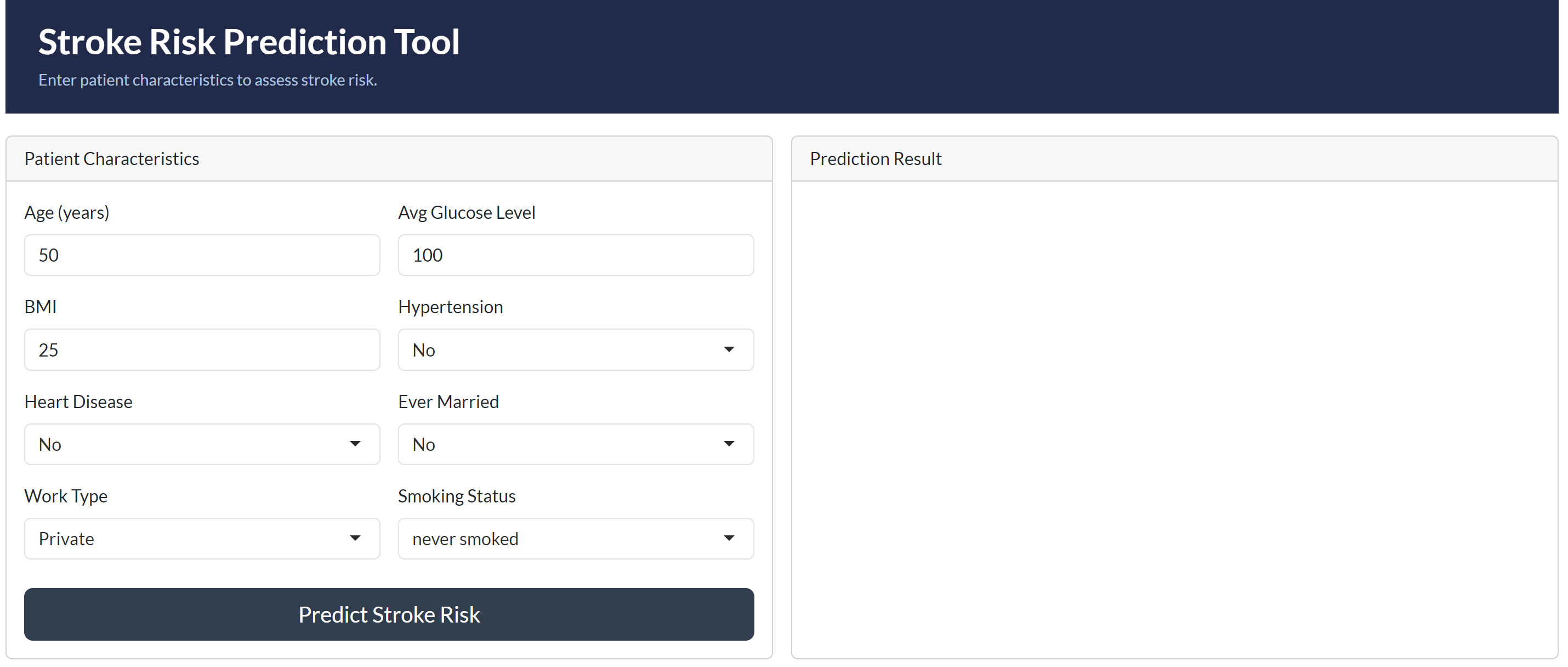
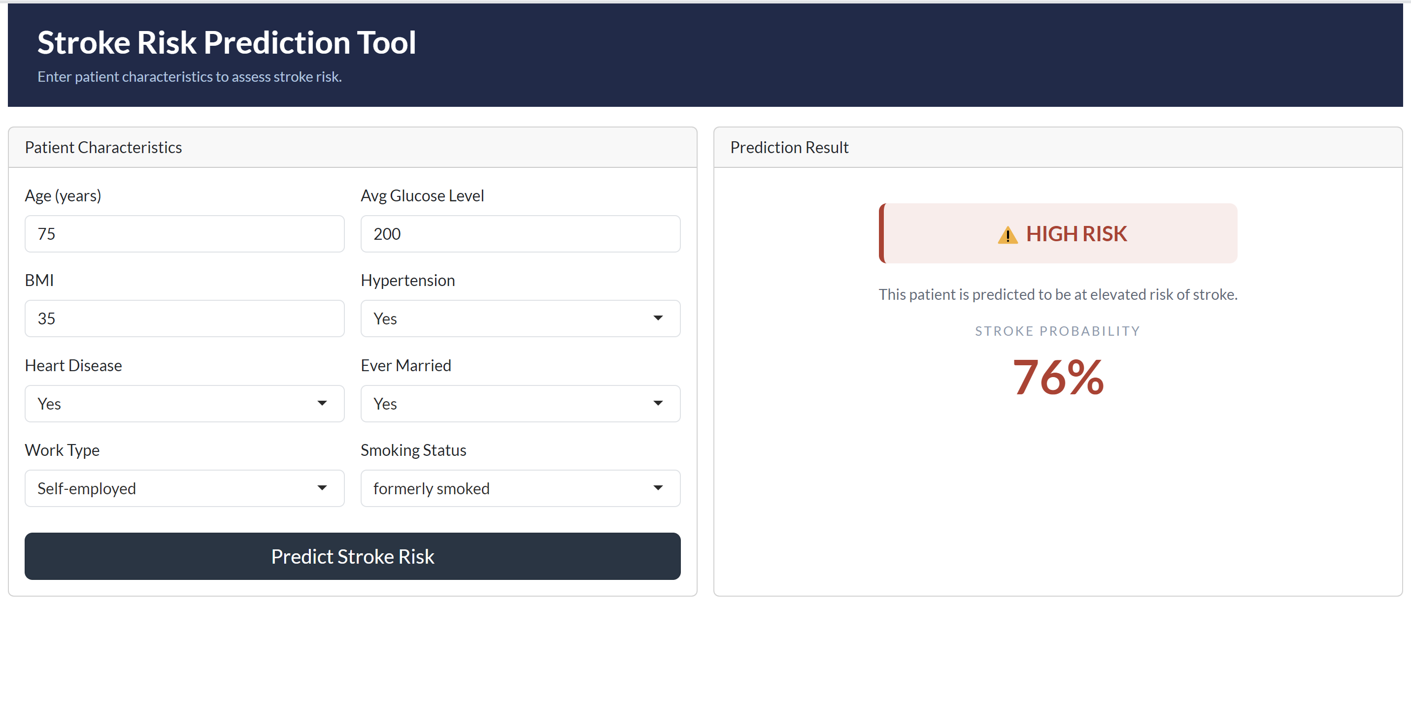
The deployed Stroke Risk Prediction Tool successfully demonstrates the model in a clinical context. When tested with a high-risk patient profile, aged 75, with hypertension, heart disease, a history of smoking, and elevated glucose levels, the model correctly returned a HIGH RISK classification with a stroke probability of 76%, a clinically coherent and expected result given the cumulative risk factors present.

The deployment is structured across two complementary layers. Vetiver packages the logistic regression model as a versioned REST API with endpoints for prediction, health monitoring, and metadata retrieval, representing how the model would be integrated into a healthcare organisation’s clinical information systems. The Shiny application provides an accessible front-end through which clinicians can input patient characteristics and receive immediate, interpretable risk assessments without requiring any technical expertise.

Together, these two components fulfil the project objective of enhancing clinical decision-making, enabling early identification of high-risk patients and supporting timely preventive intervention.

6.4.2 Shiny Application Interface

Stroke Risk Prediction Tool — Patient Input Interface

6.4.3 Shiny Application Prediction Result

Stroke Risk Prediction Tool HIGH RISK Prediction (76% Stroke Probability)

7 Task 5: Findings and Conclusions

7.1 Summary of Findings

This project set out to build and deploy a validated stroke prediction model for clinical use across 5,109 patient records. The analysis identified age, average glucose level, hypertension, and heart disease as the most significant predictors of stroke risk. Class imbalance, with only 4.87% of patients having experienced a stroke, was identified as the primary modelling challenge and addressed through SMOTE resampling during training.

Five classification models were trained, tuned, and evaluated; logistic regression, decision tree, random forest, support vector machine, and XGBoost. Logistic regression emerged as the best model, achieving the highest ROC AUC of 0.847 on the held-out test set with a clinically balanced sensitivity of 0.737 and specificity of 0.739.

7.2 Model Performance Summary

The table below summarises the final test set performance of all five models following hyperparameter tuning:

Model	Accuracy	ROC AUC	Sensitivity	Specificity
Logistic Regression	0.739	0.847	0.737	0.739
Decision Tree	0.781	0.802	0.789	0.780
Random Forest	0.892	0.818	0.386	0.922
SVM	0.717	0.836	0.772	0.714
XGBoost	0.779	0.832	0.719	0.782

Logistic regression was selected as the best model based on its superior ROC AUC and the most clinically balanced combination of sensitivity and specificity. Random forest was disqualified despite its high accuracy due to a critically low sensitivity of 0.386, correctly identifying less than 39% of actual stroke patients, rendering it clinically unsuitable regardless of its overall accuracy score.

7.3 Clinical Implications

The deployed stroke prediction model has direct and meaningful implications for clinical practice at the healthcare organisation.

Patients identified as high risk can be flagged for early intervention before a stroke event occurs, enabling clinicians to initiate preventive measures such as blood pressure management, glucose control, and lifestyle modification in a timely manner. The model’s sensitivity of 0.737 means that approximately 3 in every 4 actual stroke patients will be correctly identified and referred for early intervention.

The finding that age, hypertension, heart disease, and average glucose level are the dominant risk factors aligns with established clinical evidence and reinforces the importance of routine monitoring of these characteristics in older patient populations. The organisation can use these findings to design targeted screening programmes focused on patients above the age of 60 with one or more of these comorbidities.

The interpretability of the logistic regression model is a particular clinical asset. Unlike black-box ensemble models, logistic regression produces transparent, explainable predictions, a critical requirement for clinical adoption, patient communication, and regulatory compliance in a healthcare setting.

7.4 Limitations

Several limitations of this analysis should be acknowledged when interpreting the model’s findings and considering its clinical application.

Class imbalance: Despite SMOTE resampling, the severe 95/5 class imbalance in the dataset remains a fundamental constraint. The model was trained on a relatively small number of actual stroke cases, 248 records, which limits the richness of patterns available for the model to learn from. A larger dataset with greater stroke representation would likely produce stronger and more generalisable performance.

Missing smoking status data: A proportion of patients in the dataset had smoking status recorded as “Unknown.” This introduces uncertainty into one of the clinically relevant predictor variables and may have reduced the model’s ability to fully capture the contribution of smoking history to stroke risk.

Cross-sectional data: The dataset represents a single snapshot of patient characteristics rather than longitudinal health records. Stroke risk in clinical practice evolves over time, changes in blood pressure, glucose levels, and lifestyle factors are not captured in a static dataset, limiting the model’s ability to reflect dynamic risk trajectories.

External validity: The model was trained and evaluated on a single dataset of unknown geographic and demographic origin. Its performance on patient populations from different healthcare settings, regions, or ethnic backgrounds has not been validated and should not be assumed.

7.5 Recommendations

Based on the findings of this analysis, the following recommendations are made to the healthcare organisation:

Deploy the logistic regression model as the primary screening tool. The model’s balanced sensitivity and specificity, combined with its interpretability, make it the most suitable candidate for integration into clinical workflows. The Shiny application provides an immediate, accessible interface for frontline clinical use while the Vetiver API enables integration into existing clinical information systems.

Prioritise screening for patients aged 60 and above. Age was identified as the single strongest predictor of stroke risk in this dataset. Routine stroke risk assessments should be embedded into standard care pathways for older patients, particularly those presenting with hypertension, heart disease, or elevated glucose levels.

Implement routine glucose and blood pressure monitoring. Average glucose level and hypertension were the strongest secondary predictors of stroke risk. The organisation should ensure these measurements are consistently recorded and flagged when outside normal ranges, as they represent actionable intervention points.

Address missing smoking status data. The proportion of patients with unknown smoking status should be reduced through improved data collection practices at the point of care. Complete smoking history data would strengthen future iterations of the model.

Retrain the model periodically with new patient data. As the organisation accumulates additional patient records, the model should be retrained at regular intervals to maintain predictive accuracy and capture evolving patient demographics and risk profiles.

Validate the model on external patient populations before broader clinical rollout to assess its generalisability across different demographic groups and healthcare settings.

Stroke Prediction& Risk Modelling

1 About This Report

2 Introduction and Data Loading

2.1 Background & Objectives

2.2 The Libraries

2.3 Importing the Data

3 Data Preprocessing

3.1 Data Inspection

3.1.1 Interpretation

3.2 Data Types Validation

3.2.1 Interpretation

3.3 Data Cleaning and Transformation

3.3.1 Interpretation

3.4 Missing Values Check

3.4.1 Interpretation

3.5 Missing Data Imputation

3.5.1 Interpretation

3.6 Preprocessing Summary table

4 Exploratory Data Analysis

4.1 Stroke Outcome Distribution

4.1.1 Interpretation

4.2 Age Distribution by Stroke Outcome

4.2.1 Interpretation

4.3 Continuous Clinical Variables by Stroke Outcome

4.3.1 Interpretation

5 Build Prediction Models

5.1 Modelling Approach

5.2 Data Splitting

5.2.1 Interpretation

5.3 Feature Selection (Numeric Variable: Correlation with Stroke)

5.3.1 Interpretation

5.4 Feature Selection (Chi Test for Categorical Variables)

5.4.1 Interpretation

5.5 Preprocessing Recipe

5.5.1 Interpretation

5.6 Cross Validation Folds

5.6.1 Interpretation

5.7 Model Specifications

5.8 Model-Training

5.8.1

5.9 Model Comparison

5.9.1 Interpretation

5.10 Hyperparameter Tuning

5.11 Tuned Performance

5.11.1 Interpretation

5.12 Full Tuned Performance Across All Metrics

5.12.1 Interpretation

5.13 Finalized Models

5.14 Test Set Evaluation

5.14.1 Interpretation

5.15 Model Comparison Plot

5.15.1 Interpretation

5.16 Final Model Selection

5.16.1 Interpretation

5.17 Save Model

6 Model Deployment

6.1 Overview

6.1.1 Overview

6.2 Vetiver Deployment

6.2.1 Interpretation

6.3 Vetiver REST API

6.4 Vetiver Save Api

6.4.1 Interpretation

6.4.2 Shiny Application Interface

6.4.3 Shiny Application Prediction Result

7 Task 5: Findings and Conclusions

7.1 Summary of Findings

7.2 Model Performance Summary

7.3 Clinical Implications

7.4 Limitations

7.5 Recommendations

Stroke Prediction
& Risk Modelling